Exercise 9.1 Solution Example - Hoff, A First Course in Bayesian Statistical Methods
標準ベイズ統計学 演習問題 9.1 解答例
a)
Answer
The prior information means that the line \(\beta_1 + \beta_2 x\) should produce values between 22 and 24 when \(x\) is between 1 and 6. A little algebra shows that we need a prior distribution on \((\beta_1, \beta_2)\) such that \(\frac{98}{5} < \beta_1 < \frac{132}{5}\) and \(-\frac{2}{5} < \beta_2 < \frac{2}{5}\) with high probability. This could be done by taking \(\boldsymbol{\beta}_0 = (23, 0) \) and \(\Sigma_0 = \text{diag}\left( \left(\frac{17}{5} \right)^2, \left(\frac{1}{5} \right)^2 \right)\). For \(\nu_0\) and \(\sigma_0^2\), we could take \(\nu_0 = 2\) and \(\sigma_0^2 = 0.5\) so that the prior distribution of \(\sigma^2\) is concentrated around 0.5.
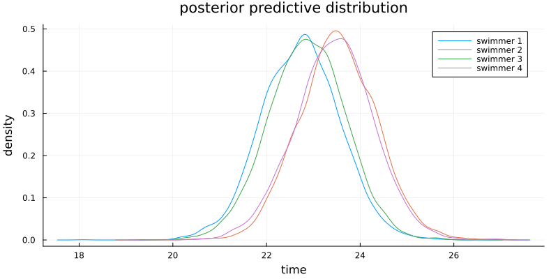
# read data
swim = readdlm("../../Exercises/swim.dat", header=false)

function regressionSemiconjugatePrior(y, X, β₀, Σ₀, ν₀, σ₀²; S=5000)
    n, p = size(X)

    BETA = Matrix{Float64}(undef, S, p)
    SIGMA² = Vector{Float64}(undef, S)

    # starting values
    olsfit = lm(X, y)
    β = coef(olsfit)
    σ² = sum(map(x -> x^2, residuals(olsfit))) / (n - p)

    # MCMC algorithm
    for s in 1:S
        # update β
        V = inv(inv(Σ₀) + X'X / σ²)
        E = V * (inv(Σ₀) * β₀ + X'y / σ²)
        β = rand(MvNormal(E, Symmetric(V)))

        # update σ²
        νₙ = ν₀ + n
        SSR = sum(map(x -> x^2, y - X*β))
        νₙσ²ₙ = ν₀ * σ₀² + SSR
        σ² = rand(InverseGamma(νₙ / 2, 2/νₙσ²ₙ))

        # store
        BETA[s, :] = β
        SIGMA²[s] = σ²
    end

    return BETA, SIGMA²
end

# set prior parameters
β₀ = [23, 0]
Σ₀ = diagm([(17/5)^2, (1/5)^2])
ν₀ = 2
σ₀² = 0.5

S = 5000

Y_PRED = Matrix{Float64}(undef, S, size(swim,1))
fig = plot(
    title="posterior predictive distribution", xlabel="time", ylabel="density"
    , size=(800, 400), margin=3mm
)
for i in 1:size(swim,1)
    y = swim[i, :]
    X = [repeat([1], length(y)) 1:length(y)]
    BETA, SIGMA² = regressionSemiconjugatePrior(y, X, β₀, Σ₀, ν₀, σ₀², S=S)
    μ_ypred = BETA[:,1] .+ BETA[:,2] * (length(y)+1)
    ypred = rand.(Normal.(μ_ypred, sqrt.(SIGMA²)))
    Y_PRED[:, i] = ypred
    fig = density!(fig, ypred, label="swimmer $i")
    ypred_mean = ypred |> mean |> x -> round(x, digits=2)
    println("swimmer $i: ", ypred_mean)
end
:RESULTS:
swimmer 1: 22.73
swimmer 2: 23.52
swimmer 3: 22.86
swimmer 4: 23.44
b)
Answer
ind_fastest = mapslices(x -> x .== minimum(x), Y_PRED, dims=2)
mean(ind_fastest, dims=1)
:RESULTS:
1×4 Matrix{Float64}:
 0.4184  0.1064  0.3504  0.1248
The probability that each swimmer is the fastest is shown above. Swimmer 1 will be the fastest with probability 0.4184, so I recommend that the coach choose swimmer 1.