Exercise 7.3 Solution Example - Hoff, A First Course in Bayesian Statistical Methods
標準ベイズ統計学 演習問題 7.3 解答例
a)
Answer
import Pkg; Pkg.activate("..")
using DelimitedFiles
using Distributions
using LinearAlgebra
using StatsBase

bluecrab = readdlm("../../Exercises/bluecrab.dat")
orangecrap = readdlm("../../Exercises/orangecrab.dat")

μ_blue = mean(bluecrab, dims=1) |> vec
μ_orange = mean(orangecrap, dims=1) |> vec

Λ_blue = S_blue = cov(bluecrab)
Λ_orange = S_orange = cov(orangecrap)

ν₀ = 4

# Gibbs sampler
function bivariate_gibbs(S, Σ_init, μ₀, Λ₀, S₀, ν₀, Y)
    THETA = Matrix{Float64}(undef, S, 2)
    SIGMA = Matrix{Float64}(undef, S, 4)
    n = size(Y, 1)
    Σ = Σ_init
    ȳ = mean(Y, dims=1) |> vec
    for s in 1:S
        # update θ
        Λn = inv( inv(Λ₀) + n * inv(Σ) )
        μn = Λn * ( inv(Λ₀) * μ₀ + n * inv(Σ) * ȳ ) |> vec
        dist = MvNormal(μn, Symmetric(Λn))
        θ = rand(dist)

        # update Σ
        Sn = S₀ + (Y' .- θ) * (Y' .- θ)'
        Σ = rand(InverseWishart(n + ν₀, Sn))

        # save results
        THETA[s, :] = vec(θ)
        SIGMA[s, :] = vec(Σ)
    end
    return THETA, SIGMA
end

S = 10000
# Blue crab
THETA_blue, SIGMA_blue = bivariate_gibbs(S, Λ_blue, μ_blue, Λ_blue, S_blue, ν₀, bluecrab)
# Orange crab
THETA_orange, SIGMA_orange = bivariate_gibbs(S, Λ_orange, μ_orange, Λ_orange, S_orange, ν₀, orangecrap)
b)
Answer
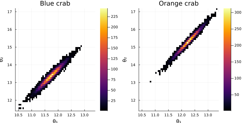
- 両方の種で、\(\theta_1\) と \(\theta_2\) は正の相関を持つ。 ( \(\theta_1\) and \(\theta_2\) have a positive correlation in both species.)
- orange crab の方が blue crab よりも幅、深さともに大きい。 (Orange crab is larger in both width and depth than blue crab.)
c)
Answer
function get_pos_cor(SIGMA, p, S)
    COR = Array{Float64}(undef, p, p, S)
    for s in 1:S
        Sig = reshape(SIGMA[s, :], p, p)
        COR[:, :, s] = Sig ./ sqrt.(diag(Sig) * diag(Sig)')
    end
    return COR
end
p = bluecrab |> size |> last
COR_mc_blue = get_pos_cor(SIGMA_blue, p, S)
COR_mc_orange = get_pos_cor(SIGMA_orange, p, S)
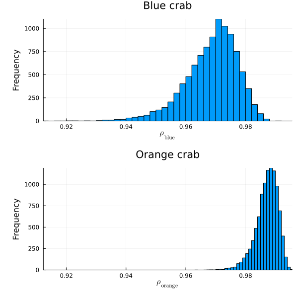
mean(COR_mc_blue[1, 2, :] .< COR_mc_orange[1, 2, :] )
0.9893
- オレンジの方がブルーに比べて、幅と深さの相関が強い。 (Orange crab has a higher correlation between width and depth than blue crab.)