Exercise 3.8 Solution Example - Hoff, A First Course in Bayesian Statistical Methods
標準ベイズ統計学 演習問題 3.8 解答例
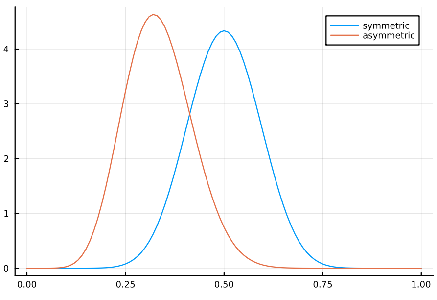
a)
answer
a₀_sym, b₀_sym = 15, 15
sym = Beta(a₀_sym, b₀_sym)
a₀_asym, b₀_asym = 10, 20
asym = Beta(a₀_asym, b₀_asym)
plot(sym, 0:0.01:1, label="symmetric")
plot!(asym, 0:0.01:1, label="asymmetric")
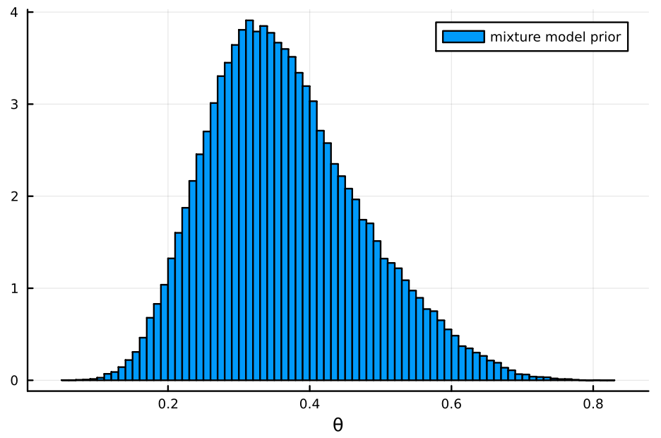
上の mixture model は、以下のようになる。
mm = MixtureModel([sym, asym], [0.2, 0.8])
histogram(rand(mm, 100000), label="mixture model prior", bins=100, normalize=:pdf, xlabel="θ")
b)
answer
| num | front |
|---|---|
| 1 | 1 |
| 2 | 1 |
| 3 | 1 |
| 4 | 1 |
| 5 | 1 |
| 6 | 0 |
| 7 | 1 |
| 8 | 0 |
| 9 | 0 |
| 10 | 1 |
| 11 | 0 |
| 12 | 0 |
| 13 | 1 |
| 14 | 0 |
| 15 | 1 |
| 16 | 1 |
| 17 | 0 |
| 18 | 0 |
| 19 | 1 |
| 20 | 0 |
| 21 | 1 |
| 22 | 0 |
| 23 | 1 |
| 24 | 0 |
| 25 | 0 |
| 26 | 0 |
| 27 | 1 |
| 28 | 0 |
| 29 | 0 |
| 30 | 1 |
| 31 | 1 |
| 32 | 0 |
| 33 | 0 |
| 34 | 0 |
| 35 | 1 |
| 36 | 1 |
| 37 | 1 |
| 38 | 0 |
| 39 | 0 |
| 40 | 1 |
| 41 | 0 |
| 42 | 0 |
| 43 | 1 |
| 44 | 0 |
| 45 | 0 |
| 46 | 0 |
| 47 | 0 |
| 48 | 1 |
| 49 | 0 |
| 50 | 1 |
| Total | 23 |
平成 26 年 100 円玉 (100 yen coin from 2014)
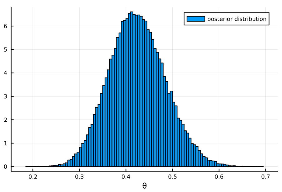
c)
answer
y₁, n₁ = 23 , 50
sym₁ = Beta(a₀_sym + y₁, b₀_sym + n₁ - y₁)
asym₁ = Beta(a₀_asym + y₁, b₀_asym + n₁ - y₁)
mm₁ = MixtureModel([sym₁, asym₁], [0.2, 0.8])
histogram(rand(mm₁, 100000), label="posterior distribution", bins=100, normalize=:pdf, xlabel="θ")
d)
answer
今回は、令和元年 100 円玉を使う。 (I will use a 100 yen coin from 2019.)
| num | front |
|---|---|
| 1 | 0 |
| 2 | 0 |
| 3 | 1 |
| 4 | 0 |
| 5 | 0 |
| 6 | 1 |
| 7 | 1 |
| 8 | 1 |
| 9 | 0 |
| 10 | 0 |
| 11 | 0 |
| 12 | 1 |
| 13 | 1 |
| 14 | 0 |
| 15 | 0 |
| 16 | 0 |
| 17 | 0 |
| 18 | 0 |
| 19 | 0 |
| 20 | 1 |
| 21 | 1 |
| 22 | 1 |
| 23 | 0 |
| 24 | 0 |
| 25 | 0 |
| 26 | 0 |
| 27 | 1 |
| 28 | 1 |
| 29 | 0 |
| 30 | 0 |
| 31 | 0 |
| 32 | 1 |
| 33 | 0 |
| 34 | 0 |
| 35 | 1 |
| 36 | 1 |
| 37 | 0 |
| 38 | 0 |
| 39 | 1 |
| 40 | 1 |
| 41 | 1 |
| 42 | 1 |
| 43 | 0 |
| 44 | 0 |
| 45 | 0 |
| 46 | 1 |
| 47 | 0 |
| 48 | 0 |
| 49 | 0 |
| 50 | 1 |
| Total | 20 |
同じ 100 円玉なので、 c) で得た事後分布を事前分布として用いると、事後分布は以下のようになる。 (Since it is the same 100 yen coin, I will use the posterior distribution obtained in c) as the prior distribution, and the posterior distribution will be as follows.)
n₂, y₂ = 50, 20
sym₂ = Beta(a₀_sym + y₁ + y₂, b₀_sym + n₁ - y₁ + n₂ - y₂)
asym₂ = Beta(a₀_asym + y₁ + y₂, b₀_asym + n₁ - y₁ + n₂ - y₂)
mm₂ = MixtureModel([sym₂, asym₂], [0.2, 0.8])
histogram(rand(mm₂, 100000), label="posterior distribution", bins=100, normalize=:pdf, xlabel="θ")
